DATAMATH CALCULATOR MUSEUM
|
|
DATAMATH CALCULATOR MUSEUM |
Even before Jack Kilby's Invention of the Integrated Circuit (IC) in September 1958, enabling Electronic Calculators as we know them today, there were already Digital Computers. While the concept of Boolean algebra, the representation of the values of variables with "true" and "false", usually denoted with 1 and 0, was known since 1847, was it Konrad Zuse developing and building from 1936 to 1938 with the Z1 the World's first freely programmable computer using binary numbers. To overcome the unreliability of this motor-driven mechanical computer, the design of the first "Electronic Numerical Integrator and Computer" better known as ENIAC, started in 1945 and was based mainly on vacuum tubes and crystal diodes for its logic. Next step of evolution, often called second-generation computer, was the introduction of fully transistorized computers mid of the 1950s and laying the foundation for Electronic Desktop Calculators. In 1964 three fully-transistorized desktop calculators arrived on the market within a few weeks: Friden EC-130, IME 84rc, and Sharp CS-10A. The EC-130 used a Cathode Ray Tube (CRT) to display 4 lines of a calculation and both IME 84rc and CS-10A used Nixie tubes, a cold cathode display, to output up to 16-digit decimal numbers in one line. Sharp's CS-10A design used a total of 530 germanium transistors and 2,300 germanium diodes and sold in 1965 for around USD 2,500 or almost US$ 25,000 in 2023 money.
The first commercially available IC, the SN502 Solid Circuit Flip Flop introduced in March 1960 for US$ 450 per unit, was not an immediate option to reduce manufacturing costs of Electronic Desktop Calculators but paved the way toward compact, reliable and affordable product. Starting in 1961 different Digital Circuits manufactured in bipolar silicon technology were introduced to the marked based on RTL (Resistor-Transistor Logic), DTL (Diode-Transistor Logic) and TTL (Transistor-Transistor Logic) leading to higher and higher complexity of the ICs and resulting in a very fast product innovation cycle. Looking in Sharp Corporation's Calculator Innovations, you'll find:
| Compet 10 (CS-10A) | World’s first all transistor-diode electronic desktop calculator | 17.0" x 16.5" x 9.8" | 55 lbs. | ¥535,000 | March 1964 | 530 transistors 2300 diodes |
| CS-031A | World’s first electronic calculator incorporating ICs | 18.9" x 15.7" x 8.7" | 29 lbs. | ¥350.000 | 1966 | 28 ICs 553 transistors 1549 diodes |
| CS-16 | World’s first calculator incorporating PMOS ICs | 13.0 x 11.5" x 5.0" | 13 lbs. | March 1967 | 72 ICs |
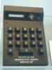
 When Jack Kilby started in 1965 together with his
colleagues Jerry D. Merryman
and James H. Van Tassel the
Cal-Tech Project, they envisioned building an IC-based,
battery-powered "miniature calculator" that could add, subtract, multiply and
divide, yet could fit in the palm of the hand. Using large and power-hungry
Nixie tubes wasn't an option for the team to display the calculating results and
they invented a technology using a dot-matrix heat element printing serially on a
roll of heat-sensitive paper. After two years of development, the three TIers
completed the first hand-held calculator in 1967. The battery-powered device
could accept six-digit numbers, perform the four basic arithmetic functions, and
print results as large as 12 digits on a thermal printer. The calculator had a
case fashioned from a solid piece of aluminum; it measure about 4-1/4 by 6-1/8
by 1-3/4 inches and weighed 45 ounces. The Cal-Tech project was meant as
"Proof-of-Concept" for so-called Large Scale Integration of Integrated Circuits
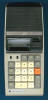
and it went well. Canon commercialized the technology developed by Texas
Instruments and introduced in 1970 with the Pocketronic the World's first
battery-powered printing calculator.
When Jack Kilby started in 1965 together with his
colleagues Jerry D. Merryman
and James H. Van Tassel the
Cal-Tech Project, they envisioned building an IC-based,
battery-powered "miniature calculator" that could add, subtract, multiply and
divide, yet could fit in the palm of the hand. Using large and power-hungry
Nixie tubes wasn't an option for the team to display the calculating results and
they invented a technology using a dot-matrix heat element printing serially on a
roll of heat-sensitive paper. After two years of development, the three TIers
completed the first hand-held calculator in 1967. The battery-powered device
could accept six-digit numbers, perform the four basic arithmetic functions, and
print results as large as 12 digits on a thermal printer. The calculator had a
case fashioned from a solid piece of aluminum; it measure about 4-1/4 by 6-1/8
by 1-3/4 inches and weighed 45 ounces. The Cal-Tech project was meant as
"Proof-of-Concept" for so-called Large Scale Integration of Integrated Circuits
and it went well. Canon commercialized the technology developed by Texas
Instruments and introduced in 1970 with the Pocketronic the World's first
battery-powered printing calculator.
In 1965,
Gordon E.
Moore - co-founder of Intel - postulated that the number of transistors that can
be packed into a given unit of space will double about every two years. This
allowed to integrate more and more transistors, diodes and resistors into
Integrated Circuits and we differentiate between "Small Scale Integration" (SSI)
with complexities in the lower tens of components, "Medium Scale Integration"
(MSI) with tens to hundreds of components on a single chip and "Large Scale
Integration" (LSI) with one thousand and more components integrated on a small
silicon chip. Looking again into Sharp Corporations' Calculator Innovations, we
basically can see that around 2,800 discrete components were reduced with the
next generation of desktop calculator to around 2,100 discrete components and 28
ICs (SSI) and the following generation used only 72 ICs (SSI and MSI). Next
major milestone for Sharp was the introduction of the QT-8D in 1969, reducing
the complexity of the design further to 6 ICs (4 LSI and 2 MSI):
| Micro Compet QT-8D | World’s first electronic calculator incorporating LSI ICs | 9.8" x 5.4" x 2.8" | 3.1 lbs. | ¥99.800 | October 1969 | 4 LSI ICs 2 MSI ICs |
The design of LSI ICs was mainly a result of switching from bipolar transistor technology to Metal-oxide Semiconductor (MOS) technology, allowing higher densities for transistors used with digital functions like logic gates and storage registers found in electronic calculators and computers. In 1969 it was commercially possible to integrate about 1,000 transistors in a p-Channel MOS (PMOS) process on a silicon die measuring about 0.2" x 0.2" (5 mm x 5 mm) and having about 28 to 48 electrical connections to the outside world. Using the equivalent of around 5,000 transistor functions for a typical electronic calculator design, most "Chipsets" for electronic calculators introduced around 1970 consisted of about 3 to 6 LSI ICs.
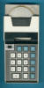
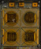
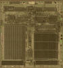
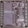 Looking
closely at the silicon die of the TMS1000, the
first commercial available Microcomputer introduced in 1974 with the
SR-10 calculator, you will notice that two
larger blocks on the die use about 50% of its real estate: The 256-bit
Random-Access Memory (RAM) at the upper left of the chip and the 8,192 Bits
Read-Only program Memory (ROM) at the lower left of the chip. In 1965 every
transistor counted and neither RAM nor ROM was an option for the earliest
electronic calculators. How do electronic calculators work? Remember how to add
two 2-digit numbers with pencil and paper? Yes, align the numbers so that the
tens' and ones' line up neatly and draw a line under them. Add the digits in the
ones' column together, if the result is larger than 10, add a one to the tens'
column. Finally add the numbers in the tens' column together and if the result
is larger than 100, add a one to the hundreds' result. And multiplications and
divisions are just simple algorithm going back to a large numbers of additions and
subtractions, respectively. This is precisely how the first electronic
calculators worked. The numbers are represented as "Binary-Coded Decimals" (BCD),
meaning 4 bits are grouped together for each digit of the number with the
individual bits having a weight of 8 (23), 4 (22), 2 (21), and 1 (20):
Looking
closely at the silicon die of the TMS1000, the
first commercial available Microcomputer introduced in 1974 with the
SR-10 calculator, you will notice that two
larger blocks on the die use about 50% of its real estate: The 256-bit
Random-Access Memory (RAM) at the upper left of the chip and the 8,192 Bits
Read-Only program Memory (ROM) at the lower left of the chip. In 1965 every
transistor counted and neither RAM nor ROM was an option for the earliest
electronic calculators. How do electronic calculators work? Remember how to add
two 2-digit numbers with pencil and paper? Yes, align the numbers so that the
tens' and ones' line up neatly and draw a line under them. Add the digits in the
ones' column together, if the result is larger than 10, add a one to the tens'
column. Finally add the numbers in the tens' column together and if the result
is larger than 100, add a one to the hundreds' result. And multiplications and
divisions are just simple algorithm going back to a large numbers of additions and
subtractions, respectively. This is precisely how the first electronic
calculators worked. The numbers are represented as "Binary-Coded Decimals" (BCD),
meaning 4 bits are grouped together for each digit of the number with the
individual bits having a weight of 8 (23), 4 (22), 2 (21), and 1 (20):
| Decimal | 23 | 22 | 21 | 20 | BCD |
| 0 | 0 | 0 | 0 | 0 | 0b0000 |
| 1 | 0 | 0 | 0 | 1 | 0b0001 |
| 2 | 0 | 0 | 1 | 0 | 0b0010 |
| 3 | 0 | 0 | 1 | 1 | 0b0011 |
| 4 | 0 | 1 | 0 | 0 | 0b0100 |
| 5 | 0 | 1 | 0 | 1 | 0b0101 |
| 6 | 0 | 1 | 1 | 0 | 0b0110 |
| 7 | 0 | 1 | 1 | 1 | 0b0111 |
| 8 | 1 | 0 | 0 | 0 | 0b1000 |
| 9 | 1 | 0 | 0 | 1 | 0b1001 |
 Using now a 4-bit Binary Adder with two BCD
numbers results for example with 3 + 5 as operands to the expected result of: 0b0011 + 0b0101 =
0b1000 or decimal 8. But trying to add 5 + 7 results in 0b0101 + 0b0111 = 0b1100 which
is not defined as a BCD number. BCD-Adders detect this kind of overflow and
correct the result by adding the constant 6 to the interims result, giving 0b1100 + 0b0110 =
0b10010 with the leftmost bit as a carry over into the digit to the left
and finally resulting in 0b00010010 or decimal 12. Adding now two large 12 digit
numbers would not necessarily require a 48-bit Binary Adder, the numbers are added digit by
digit, from the right to the left. Actual implementations sometimes even
substitute the 4-bit Adder with a 1-bit Adder used 4-times in a loop per digit.
Hewlett Packard's innovative HP-35
is representing numbers with 56 bits, divided into 4 bits for the sign of the
mantissa, 40 bits for the mantissa, 4 bits for the sign of the exponent, and 8
bits for the exponent and using a 1-bit Adder for a bit-serial architecture
versus digit-serial architectures using a 4-bit Adder.
Using now a 4-bit Binary Adder with two BCD
numbers results for example with 3 + 5 as operands to the expected result of: 0b0011 + 0b0101 =
0b1000 or decimal 8. But trying to add 5 + 7 results in 0b0101 + 0b0111 = 0b1100 which
is not defined as a BCD number. BCD-Adders detect this kind of overflow and
correct the result by adding the constant 6 to the interims result, giving 0b1100 + 0b0110 =
0b10010 with the leftmost bit as a carry over into the digit to the left
and finally resulting in 0b00010010 or decimal 12. Adding now two large 12 digit
numbers would not necessarily require a 48-bit Binary Adder, the numbers are added digit by
digit, from the right to the left. Actual implementations sometimes even
substitute the 4-bit Adder with a 1-bit Adder used 4-times in a loop per digit.
Hewlett Packard's innovative HP-35
is representing numbers with 56 bits, divided into 4 bits for the sign of the
mantissa, 40 bits for the mantissa, 4 bits for the sign of the exponent, and 8
bits for the exponent and using a 1-bit Adder for a bit-serial architecture
versus digit-serial architectures using a 4-bit Adder.
 The
above mentioned 256-bit RAM of the TMS1000 would be capable of storing up to 4
numbers of 16-digit length but has an extremely high transistor count due to its
design and implementation. Early transistorized calculators used a completely
different approach to store numbers, Friden's EC-130 for examples used a magnetostrictive delay line, an acoustic delay line technology tracing back to the mercury delay lines pioneered in the 1950s, a truly serial type of storage.
The electronic equivalent of delay lines are shift registers and with the advent
of MOS LSI technology, shift registers were actually the first mass-produced
PMOS chips starting in 1964 with 20 bits and
leading within a few years to densities of hundreds of bits. Texas Instruments
Cal-Tech demonstrator used for storage of the numbers three shift registers and
divided the remaining electronics into four logic chip and their approach proved
correct, dynamic and later static shift registers dominated the design of
electronic calculators in their infancy, hitting the sweet spot of high
integration density and application match of serial architectures. The resulting
memory configuration is called Serial Access Memory (SAM) and the numbers are
stored like on a racetrack and always circling, contrary to RAM where every bit
can be accessed in a random order.
The
above mentioned 256-bit RAM of the TMS1000 would be capable of storing up to 4
numbers of 16-digit length but has an extremely high transistor count due to its
design and implementation. Early transistorized calculators used a completely
different approach to store numbers, Friden's EC-130 for examples used a magnetostrictive delay line, an acoustic delay line technology tracing back to the mercury delay lines pioneered in the 1950s, a truly serial type of storage.
The electronic equivalent of delay lines are shift registers and with the advent
of MOS LSI technology, shift registers were actually the first mass-produced
PMOS chips starting in 1964 with 20 bits and
leading within a few years to densities of hundreds of bits. Texas Instruments
Cal-Tech demonstrator used for storage of the numbers three shift registers and
divided the remaining electronics into four logic chip and their approach proved
correct, dynamic and later static shift registers dominated the design of
electronic calculators in their infancy, hitting the sweet spot of high
integration density and application match of serial architectures. The resulting
memory configuration is called Serial Access Memory (SAM) and the numbers are
stored like on a racetrack and always circling, contrary to RAM where every bit
can be accessed in a random order.
The other large block of the TMS1000 is its 8,192 Bits ROM to store the program of the calculator, like scanning the keyboard, controlling the display, managing the registers for the adders and many more tasks. Well, there are differences between computers and calculators and early electronic calculators didn't use any program memory. In the early days of Electronic Calculators, it was all about transistor count - with fully-transistorized calculators it defined the manufacturing costs, product size, power consumption, reliability and competitiveness while with LSI technology it defined how many (expensive) PMOS ICs the calculator design would need. To reduce transistor count to the bare minimum, their was no programmability at the beginning - everything was "hard-coded" in the chip design. Advantage of low transistor count was disadvantage of inflexible designs and following Moore's Law within a few years two major changes took place:
|
• From Multi-Chip Designs to Single-Chip Designs • From Register Processors to Digit Processors |
 The first bullet point addresses improvements in
the topology of "Calculator Chipsets" and the second bullet point addresses
improvements of the flexibility of the calculator designs. Starting with the
Cal-Tech demonstrator in 1965, it required four large PMOS ICs for the
calculator logic and three smaller PMOS ICs for the shift registers to store
three numbers (Input register, Output register, Interims calculation register).
"Slicing" the calculator design was based on two factors: Number of transistors
per chip and numbers of connections per chip. The Pocketronic introduced in
April 1970 divided the electronics into three PMOS ICs with 40-pin and 28-pin
packages while the Canon L121 introduced in 1971 needed a forth chip for its
Nixie tube display.
The first bullet point addresses improvements in
the topology of "Calculator Chipsets" and the second bullet point addresses
improvements of the flexibility of the calculator designs. Starting with the
Cal-Tech demonstrator in 1965, it required four large PMOS ICs for the
calculator logic and three smaller PMOS ICs for the shift registers to store
three numbers (Input register, Output register, Interims calculation register).
"Slicing" the calculator design was based on two factors: Number of transistors
per chip and numbers of connections per chip. The Pocketronic introduced in
April 1970 divided the electronics into three PMOS ICs with 40-pin and 28-pin
packages while the Canon L121 introduced in 1971 needed a forth chip for its
Nixie tube display.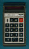 The Bowmar 901B introduced in September
1971 was based on a single-chip calculator circuit encapsulated in a 28-pin
package but still using a Register-Architecture similar to the Cal-Tech design.
Texas Instruments as a leading manufacturer of Calculator
Chipsets for customers like Canon, Smith Corona Marchant, Olivetti and
Sumlock Compucorp observed early in the 1970s that every customer design was
unique but yet pretty similar to other designs and they started to add some
flexibility to their designs, allowing for shorter design cycles and lower
design costs. Instead of "slicing" complete designs randomly into pieces that
met the criteria of die size and pin count they restructured the calculator
designs into "Building Blocks" that could be arranged like Legos and implemented
some programmability in ROM structures for the algorithm and Programmable Logic
Array (PLA) structures for logic, like segment decoder or display timing and
polarity. Main difference between "Multi-Chip Slices" and "Building Blocks" is
the approach how the partitioning of a given calculator design takes place.
"Slicing" takes place on the gate level or transistor level of the calculator
schematics and implementation of the design with the least possible number of
silicon dies is the main motivation. Creating "Building Blocks" happens one
layer above, on block diagram level and reuse of the resulting silicon dies is
here the main driver. Building Blocks make the chips itself more complicated by
adding well defined "connectors" to every single block, similar to Legos
blocks. While in early Multi-Chip designs as an example one chip was responsible
for the overall timing of the system and broadcasted its current state on
typically 4 signals, generates every TMS0500 Building Block its own timing and
synchronizes it to the "Master Timing" of the TMC0501. Even the clock oscillator
of a TI-59 recognizes if the calculator brain is just scanning the keyboard or
crunching numbers and adjusts its oscillation speed accordingly.
The Bowmar 901B introduced in September
1971 was based on a single-chip calculator circuit encapsulated in a 28-pin
package but still using a Register-Architecture similar to the Cal-Tech design.
Texas Instruments as a leading manufacturer of Calculator
Chipsets for customers like Canon, Smith Corona Marchant, Olivetti and
Sumlock Compucorp observed early in the 1970s that every customer design was
unique but yet pretty similar to other designs and they started to add some
flexibility to their designs, allowing for shorter design cycles and lower
design costs. Instead of "slicing" complete designs randomly into pieces that
met the criteria of die size and pin count they restructured the calculator
designs into "Building Blocks" that could be arranged like Legos and implemented
some programmability in ROM structures for the algorithm and Programmable Logic
Array (PLA) structures for logic, like segment decoder or display timing and
polarity. Main difference between "Multi-Chip Slices" and "Building Blocks" is
the approach how the partitioning of a given calculator design takes place.
"Slicing" takes place on the gate level or transistor level of the calculator
schematics and implementation of the design with the least possible number of
silicon dies is the main motivation. Creating "Building Blocks" happens one
layer above, on block diagram level and reuse of the resulting silicon dies is
here the main driver. Building Blocks make the chips itself more complicated by
adding well defined "connectors" to every single block, similar to Legos
blocks. While in early Multi-Chip designs as an example one chip was responsible
for the overall timing of the system and broadcasted its current state on
typically 4 signals, generates every TMS0500 Building Block its own timing and
synchronizes it to the "Master Timing" of the TMC0501. Even the clock oscillator
of a TI-59 recognizes if the calculator brain is just scanning the keyboard or
crunching numbers and adjusts its oscillation speed accordingly.
Here at the Datamath Calculator Museum we differentiate for calculators using Register Processors
six steps of evolution from the Cal-Tech design:
|
• 1970:
TMC1730-1732 (Canon Pocketronic): Multi-Chip Slices • 1971: TMC1813,1814 (Canon L121F): Two-Chip Slices • 1971: TMS0100 (Standard): Single-Chip Calculator Circuit • 1972: TMS0200 (Standard): Building Blocks for Desktop and Printing Calculators • 1974: TMC0500 (Standard): Building Blocks for Scientific Calculators • 1977: TMC0920, TMC1500 (Standard): Real Single-Chip Calculator Circuit including Display Drivers |
 The flexible design concept of the
TMS0100 with both programmable PLA and ROM
techniques allowed for easy individualizations and hundreds of pocket
calculators and small desktop calculators used one of its 28 known chip
variations and the groundbreaking modular approach of the
TMS0200 Building Blocks was further optimized
with the TMC0500 Building Blocks leading to the
TI-59 and being remembered for
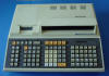
eternity. The eclipse of TMS0200 and TMC0500 Building Blocks was clearly the
SR-60 Programmable Prompting Desktop Calculator
with integrated Printer introduced in 1976 and using in its base configuration
fifteen Building Blocks. The last Register Processor developed by Texas
Instruments was the TMC1500 introduced in 1977
and not only integrating the equivalent of three TMC0500 Building Blocks but the
Display Drivers, too on a small silicon die and featuring about 30,000
transistors.
The flexible design concept of the
TMS0100 with both programmable PLA and ROM
techniques allowed for easy individualizations and hundreds of pocket
calculators and small desktop calculators used one of its 28 known chip
variations and the groundbreaking modular approach of the
TMS0200 Building Blocks was further optimized
with the TMC0500 Building Blocks leading to the
TI-59 and being remembered for
eternity. The eclipse of TMS0200 and TMC0500 Building Blocks was clearly the
SR-60 Programmable Prompting Desktop Calculator
with integrated Printer introduced in 1976 and using in its base configuration
fifteen Building Blocks. The last Register Processor developed by Texas
Instruments was the TMC1500 introduced in 1977
and not only integrating the equivalent of three TMC0500 Building Blocks but the
Display Drivers, too on a small silicon die and featuring about 30,000
transistors.
But the Register Processors inherited a disadvantage from its roots tracing back to the earliest, fully-transistorized Electronic Calculators - the shift register based Sequential Access Memory. While the sequential access of the individual digits of numbers represented in BCD format works perfectly to add large numbers, did it block the use of the chips for other applications. Single-chip calculators could add numbers but they could not keep time, control a furnace or do anything else - like a flexible microcomputer could do.
Texas Instruments realized these limitations rather quickly and the successor of the TMS0100 "calculator on a chip" was announced in 1974 as TMS1000 "computer on a chip". Comparing both the TMS0100 and TMS1000 reveals many similarities but one massive difference: The 182-bit Serial-Access Memory (SAM, 3 Registers * 13 Digits, 2 * 13 Bit-Flags) was replaced with a 256-bit Random-Access Memory and the 3,520 Bits Read-Only program Memory (ROM, 320 Words x 11 Bits) was increased to 8,192 Bits (1,024 Words x 8 Bits) and the TMS1000 Microcomputer Family took the World in a storm and was the most successful 4-bit design ever. Well, designing calculators with a Digit Processor introduced new challenges! Register Processors could add two large BCD numbers with just one instruction on the fly and Digit Processors literally need to pick one digit from one operand, one digit from the other operand, add them together, store the result back, load the next digits form the first operand and so on. Sounds time consuming? It is time consuming and Texas Instruments learned its lesson the hard way when trying with "Project X", started 1977 and abandoned in 1982, to replace the TI-59 based on a TMS0501E Register Processor introduced in 1974 with the TI-88 based on two TP0485 Digit Processors. But here Moore's Law is fortunate, too. Integrated Circuits did not only double their transistor count every two year, their clock frequency and operating speed is increasing at an almost similar rate and we are not aware of any Register Processor developed after the 1977 by Texas Instruments. Switching to flexible Digit Processors allowed designers suddenly to work not only with serial adders on long BCD numbers, they could do completely different operations on any data that could be represented and stored in the RAM of the devices like the famous Little Professor Educational Toy, the groundbreaking Speak & Spell or the TI-2000 Time Manager.
 The ongoing battle of adding new features to the next product before Moore's Law
allowed Single-Chip solutions, created with Digit Processors some Multi-Chip
designs, most notably architectures using a Main-CPU and one or more
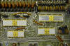
Support-CPUs. A very good example is the TI-5050
Printing Calculator introduced in March 1975 and using two Digit Processors of
the TMS1000 Series, one for keyboard scanning, calculations and display output
and a second one for the thermal printer. The TI-5050 was replaces after only 15
months with the TI-5050M, adding a User
Memory to the feature set of the TI-5050 and selling for $129.95 versus the
$199.95 price tag of its predecessor. Dismantling the TI-5050M reveals a
Single-Chip design based on the TMS1115,
basically a TMS1000 with double the RAM cpacity and double the ROM capacity of the
original TMS1000. Other
examples of Multi-Chip designs with Digit processors include the
TI-55-II introduced in 1981 with two
TP0455 chips and the
PC-800 Printer using a tandem of TMS1000
and TMS1300 Microcomputers.
The ongoing battle of adding new features to the next product before Moore's Law
allowed Single-Chip solutions, created with Digit Processors some Multi-Chip
designs, most notably architectures using a Main-CPU and one or more
Support-CPUs. A very good example is the TI-5050
Printing Calculator introduced in March 1975 and using two Digit Processors of
the TMS1000 Series, one for keyboard scanning, calculations and display output
and a second one for the thermal printer. The TI-5050 was replaces after only 15
months with the TI-5050M, adding a User
Memory to the feature set of the TI-5050 and selling for $129.95 versus the
$199.95 price tag of its predecessor. Dismantling the TI-5050M reveals a
Single-Chip design based on the TMS1115,
basically a TMS1000 with double the RAM cpacity and double the ROM capacity of the
original TMS1000. Other
examples of Multi-Chip designs with Digit processors include the
TI-55-II introduced in 1981 with two
TP0455 chips and the
PC-800 Printer using a tandem of TMS1000
and TMS1300 Microcomputers.
 Texas
Instruments' ambitious LCD III
Project proposed in January 1978 replacing all Register Processors used in their
calculator portfolio with a family of three modular Digit Processors, differing
mainly in ROM and RAM capacity and each chip optionally including additional
modules for timekeeping functions and LC-Displays drivers. Well, the project
didn't went well and the (failed) TP0485 was the last
Digit Processor that Texas Instrument developed for Electronic Calculators, with
a RAM capacity of 1,408 Bits and a ROM capacity of 41,800 Bits it was a fivefold
improvement over the original TMS1000. Texas Instruments decided to work for
future calculator chip designs with Toshiba and
most of their calculators introduced in the 1980s use 4-bit Toshiba
Microcomputer.
Texas
Instruments' ambitious LCD III
Project proposed in January 1978 replacing all Register Processors used in their
calculator portfolio with a family of three modular Digit Processors, differing
mainly in ROM and RAM capacity and each chip optionally including additional
modules for timekeeping functions and LC-Displays drivers. Well, the project
didn't went well and the (failed) TP0485 was the last
Digit Processor that Texas Instrument developed for Electronic Calculators, with
a RAM capacity of 1,408 Bits and a ROM capacity of 41,800 Bits it was a fivefold
improvement over the original TMS1000. Texas Instruments decided to work for
future calculator chip designs with Toshiba and
most of their calculators introduced in the 1980s use 4-bit Toshiba
Microcomputer.
Here at the Datamath Calculator Museum we differentiate for calculators using Digit Processors five steps of evolution from the SR-16 based on the TMS1000:
|
• 1974:
TMS1000 (Standard): Single-Chip Calculator Circuit • 1975: TMS0950 (Standard): Real Single-Chip Calculator Circuit including Display Drivers • 1975: TMS1X00 (Standard): Dual-Chip Calculator Circuit • 1978: TP0320 (Standard): Single-Chip Calculator Circuit CMOS • 1981: TP0455, TP0485 (Standard): Multi-Chip Calculator Circuit CMOS |
The next major step in evolution was switching for Graphing Calculators to 8-bit Architectures with Processors like the Z80 and external RAM and ROM. The TI-81 introduced in 1990 is centered around a Toshiba T6A49A Application-specific 8-bit Z80 CPU, 128k Bytes Mask ROM, 8k Bytes Static RAM (SRAM) and three display drivers from Toshiba for the 64 * 96 pixel dot matrix LC-Display. This basic architecture branched into three product lines before being replaced in 1999 by the TI-83 Plus architecture using more flexible Flash ROM instead the Mask ROM:
|
• 1990:
TI-81,
TI-82, TI-83,
TI-82 STATS • 1992: TI-85, TI-86 • 1995: TI-80 |
Learn more about the Hardware Architecture of TI’s Graphing Calculators.
![]()
If you have additions to the above article please email: joerg@datamath.org.
© Joerg Woerner, September 9, 2023. No reprints without written permission.